Previous - 3.6 Comparing Components of Uncertainty Index Next - 4 Presentation of Uncertainty

3.7 Estimates of Total Uncertainty

Smith and Reynolds [2005] attempted to combine all the different uncertainties described above to get a total uncertainty estimate. They combined their analysis uncertainty with measurement uncertainty, bias uncertainty and structural uncertainty. Uncertainty associated with pervasive systematic errors and structural uncertainty in the adjustments were estimated by taking the mean squared difference between the Smith and Reynolds [2002] and Folland and Parker [1995] bias adjustments in the prewar period. After World War 2, the bias uncertainty was estimated by calculating the average difference between engine room measurements and all measurements. Structural uncertainties were estimated by analysing the spread of three SST analyses.

Figure 9 shows the total uncertainty estimate from the latest version of the ERSST analysis, ERSSTv3b, in blue. A similar estimate was made based on the HadSST3 data set in the following way. Measurement uncertainties, grid-box sampling uncertainties and large-scale sampling uncertainties were estimated using the method of Kennedy et al. [2011b, 2011c]. To estimate the uncertainty associated with pervasive systematic errors,an ensemble of 200 data sets, comprising the 100 original ensemble members from HadSST3 and a 100-member ensemble generated by replacing the Rayner et al. [2006] bucket-correction fields with the fields from Smith and Reynolds [2002]. The adjustment uncertainties on individual months were assumed to be correlated within a year, giving a greater uncertainty range than in Kennedy et al. [2011c], particularly before 1941. During the war years 0.2 K was added to reflect the additional uncertainty during that period as described by Kennedy et al. [2011c]. As above, structural uncertainties were estimated by taking the standard deviation of area-average time series from seven analyses.

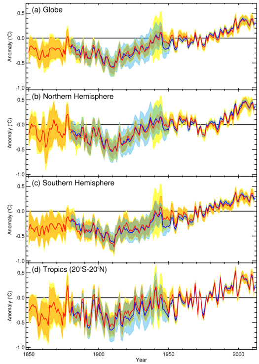
Figure 9: (a) Global, (b) Northern Hemisphere, (c) Southern Hemisphere and (d) Tropical average sea-surface temperature anomalies with estimated 95% confidence range for ERSSTv3b (1880-2012 dark blue line and pale blue shading) and for the HadSST3 based analysis described in section 3.5 (1850-2011 red line and orange and yellow shading). The yellow shading indicates an estimate of the additional structural uncertainty in the HadSST3 series.

The total uncertainty estimates from these two assessments are comparable between 1880 and 1915. Between 1915 and 1941, the ERSSTv3b uncertainty estimate is larger because the estimated bias uncertainty is larger. The difference is most obvious in the northern hemisphere where the differences between the Smith and Reynolds [2002] and Folland and Parker [1995] bias adjustments are largest. From 1941 to present, the HadSST3-based uncertainty estimate is the larger because the bias uncertainty is larger than in ERSSTv3b.

The obvious question that arises is "do these assessments span the full uncertainty range?" In this case, it probably pays to err on the side of caution. Although the structural uncertainty is based on a range of methods for infilling missing data, there are still commonalities in the approaches taken and there is little diversity in the approaches to bias adjustment. The lack of diversity is troubling because the differences between the median estimates of HadSST3 and ERSSTv3b are greater than the estimated uncertainties of the ERSSTv3b analysis at times during the period 1950-1970 suggesting that the uncertainties may have been underestimated in the earlier assessment.

Previous - 3.6 Comparing Components of Uncertainty Index Next - 4 Presentation of Uncertainty