Previous - 3.5.4 Summary of Reconstruction Techniques and Structural Uncertainty Index Next - 3.7 Estimates of Total Uncertainty

3.6 Comparing Components of Uncertainty

Figure 7 shows individual components of the overall uncertainty estimated for three months. The components include: estimates of structural uncertainty (in lieu of a formal way to estimate this, it is calculated as the standard deviation of seven near-globally-complete analyses: COBE, Kaplan, ERSSTv3, HadISST, GPFA, GP and VBPCA), sampling uncertainty, combined uncorrelated and systematic measurement error uncertainty, bias uncertainty (estimated from a 200-member ensemble described in section 4) and analysis uncertainties from ERSSTv3b [Smith et al. 2008].

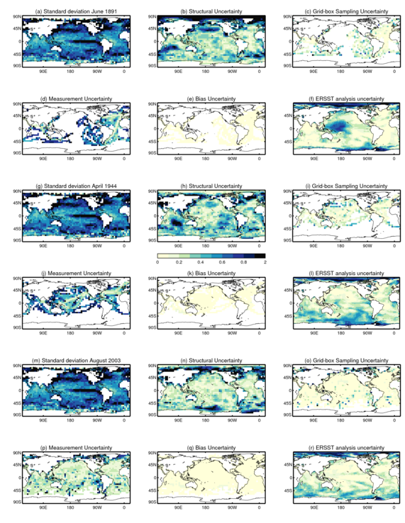
Figure 7: Maps showing climatological standard deviation of SST (a, g, m), Structural uncertainty (b, h, n), Sampling uncertainty (c, i, o), measurement uncertainty (d, j, p), bias uncertainty (e,k,q) and analysis uncertainty from ERSSTv3b (f, l, r). Three months are shown: (a-f) June 1891, (g-l) April 1944 and (m-r) August 2003.

At a monthly, grid-box level, the parametric uncertainty in the Kennedy et al. [2011c] systematic error estimates is typically the smallest uncertainty and is nearly always less than 0.2 K. The sampling uncertainty and measurement uncertainty both depend on the number of observations, so they are larger in areas with fewer observations. Of the two, measurement uncertainty is typically larger.

In well-observed periods, the spread between the different analyses is roughly what one might expect: closer agreement in well-observed regions, poorer agreement in data-sparse regions, principally the Southern Ocean and Arctic Ocean. At more poorly-observed times, the spread between analyses is narrower than the climatological standard deviation suggesting that the reconstructions are skilful in the sense that they are providing useful information in data voids. However, the narrow spread is in contrast to those areas where there have been changes in the input observations (see, for example, the Indian Ocean in Figure 7(b) and Figure 7(h)). A small number of observations, which are available to one analysis but not another, lead to a larger spread than is seen in data-free regions implying that, while there is diversity in the approaches, there may still be too little for the best estimates alone to effectively bracket the true uncertainty range.

The ERSSTv3 analysis uncertainties are largest in regions where there are consistent data voids. They show a similar pattern to the structural uncertainty estimate in 1944 and 2003, but there is marked difference in 1891, with the analysis uncertainty being larger than the structural uncertainty in the poorly-observed western Pacific.

Figure 8 shows time series of the different components of uncertainty at different spatial scales from global to grid box. The bias uncertainty is relatively constant and is the smallest component of uncertainty at the grid box level for much of the record. The sampling uncertainty for a grid box is larger than the bias uncertainty when observations are few, but in the recent record they are comparable. In this example, the measurement uncertainty is larger than bias and sampling uncertainties at the grid box level, even when observations are numerous. However, in other grid boxes, characterised by strong SST gradients or high variability, such as the western boundary currents, the sampling uncertainty could be larger.

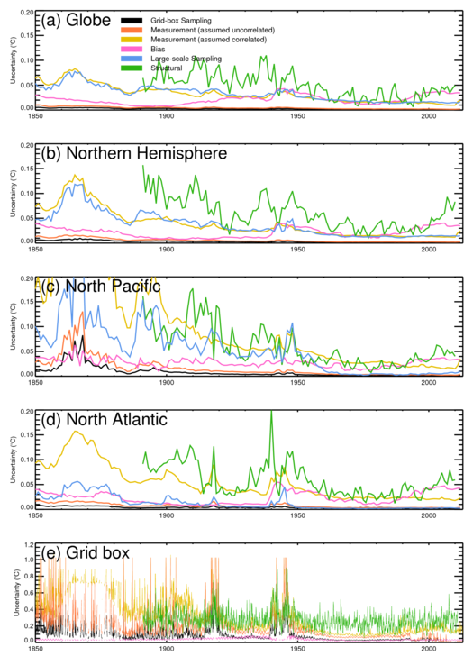
Figure 8: Time series of estimated uncertainties arising from different sources in area-averages: (a) Global annual, (b) Northern hemisphere annual, (c) North Pacific annual, (d) North Atlantic annual and (e) a 5-degree grid box centered on 42.5°W, 27.5°N monthly. Uncertainty components shown are: (pale blue) grid-box sampling uncertainty, (green) uncorrelated measurement uncertainty, (red) correlated measurement uncertainty, (dark blue) parametric bias uncertainty from a 200-member ensemble based on HadSST3, (black) large-scale sampling uncertainty, and (magenta) structural uncertainty estimated by taking the range of the area-average calculated from seven near-globally-complete analyses.

As the size of the area increases and more observations are included in the average, the sampling and measurement uncertainties decrease. Two estimates of the measurement uncertainty are included. In one, correlations between individual errors are taken into account. In the other, measurement errors are assumed to be uncorrelated and independent. In the latter case, the measurement uncertainties become small relative to other sources of uncertainty at a basin scale early in the 20th century. However, the effect of correlated errors is such that measurement uncertainty remains a major source of uncertainty at all scales until the 1980s when the global VOS fleet reached its peak and the deployment of drifting and moored buoys began.

The largest component at the scales shown here is the structural uncertainty. In the grid box shown, the structural uncertainty is, at times, larger than the combined uncertainty from other components suggesting that some or all of the analyses are losing information. At a global level, where estimated analysis uncertainties are available for COBE, COBE-2, Kaplan and ERSSTv3b data sets, the structural uncertainty is comparable to the estimated analysis uncertainties. For example, in 1900, the ERSSTv3b analysis uncertainty is 0.03K, the COBE analysis uncertainty is 0.06K, COBE-2 gives 0.05K and Kaplan is around 0.05K.

Because of the nature of the uncertainties arising from the adjustments for pervasive systematic errors, the uncertainties become relatively more important as the averaging scale increases. At a global scale, bias uncertainties are comparable to or larger than all other uncertainty components from the 1940s to the present. There is a caveat: because the SSTs are expressed as anomalies, the size of the bias uncertainty depends on the base period used to calculate the anomalies. In Figure 8, the period used is 1961-1990, which is why there is a local minimum in the bias uncertainty centred on that period.

Previous - 3.5.4 Summary of Reconstruction Techniques and Structural Uncertainty Index Next - 3.7 Estimates of Total Uncertainty