Previous - 3.4.1 Grid-box Sampling Uncertainty Index Next - 3.4.3 Summary of Sampling Uncertainty

3.4.2 Large-scale Sampling Uncertainty

Because Rayner et al. [2006] and Kennedy et al. [2011b] make no attempt to estimate temperatures in grid boxes which contain no observations, an additional uncertainty had to be computed when estimating area-averages. Rayner et al. [2006] used Optimal Averaging (OA) as described in Folland et al. [2001] which estimates the area average in a statistically optimal way and provides an estimate of the large-scale sampling uncertainty. Kennedy et al. [2011b] subsampled globally complete fields taken from three SST analyses and obtained similar uncertainties from each. The uncertainties of the global averages computed by Kennedy et al. [2011b] were generally larger than those estimated by Rayner et al. [2006]. Palmer and Brohan [2011] used an empirical method based on that employed for grid-box averages in Rayner et al. [2006] to estimate global and ocean basin averages of subsurface temperatures.

The Kennedy et al. [2011b] large-scale sampling uncertainty of the global average SST anomaly is largest (with a 2-sigma uncertainty of around 0.15K) in the 1860s when coverage was at its worst (Figure 8). This falls to 0.03K by 2006. The fact that the large-scale sampling uncertainty should be so small particularly in the nineteenth century may be surprising. The relatively small uncertainty might simply be a reflection of the assumptions made in the analyses used by Kennedy et al. [2011b] to estimate the large-scale sampling uncertainty. Indeed, Gouretski et al. [2012] found that subsampling an ocean reanalysis underestimated the uncertainty when the coverage was very sparse. However, estimates made by Jones [1994] suggest that a hemispheric-average land-surface air temperature series might be constructed using as few as a 109 stations. For SST, the variability is typically much lower than for land temperatures though the area is larger. It seems likely that the number of stations needed to make a reliable estimate of the global average SST anomaly would not be vastly greater.

Another way of assessing the large-scale sampling uncertainty is to look at the effect of reducing the coverage of well-sampled periods to that of the less-well-sampled nineteenth century and recomputing the global average (see for example Parker [1987]). Figure 4 shows the range of global annual average SST anomalies obtained by reducing each year to the coverage of years in the nineteenth century. So, for example, the range indicated by the blue area in the upper panel for 2006 shows the range of global annual averages obtained by reducing the coverage of 2006 successively to that of 1850, 1851, 1852... and so on to 1899. The red line shows the global average SST anomaly from data that have not been reduced in coverage. For most years, the difference between the sub-sampled and more fully sampled data is smaller than 0.15K and the largest deviations are smaller than 0.2K. For the large-scale sampling uncertainty of the global average to be significantly larger would require the variability in the nineteenth century data gaps to be different from that in the better-observed period.

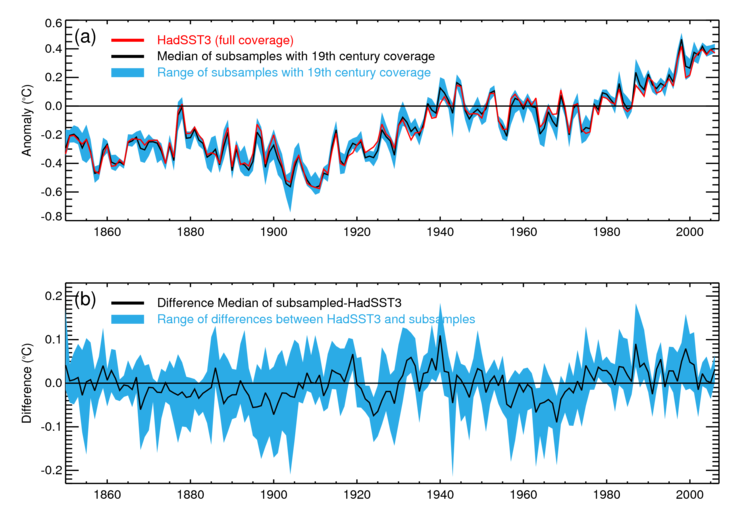
Figure 4: (a) Estimated global average SST anomaly from HadSST3 [Kennedy et al. 2011b, 2011c] (red) and for subsamples of the HadSST3 dataset reduced to 19th century coverage. The black line is the median of the samples and the blue area gives the range. (b) difference, on an expanded temperature scale, between the global average SST anomaly from the full HadSST3 data set and global averages calculated from the subsamples.

Previous - 3.4.1 Grid-box Sampling Uncertainty Index Next - 3.4.3 Summary of Sampling Uncertainty