Previous - 3.3.4 Refinements to Estimates of Pervasive Systematic Errors Index Next - 3.3.6 Summary of Pervasive Systematic Errors and Biases

3.3.5 Assessing the Efficacy of Bias Adjustments

The efficacy of the bias adjustments and their uncertainties are difficult to assess, particularly earlier in the record when there are fewere independent strands of information. There are various ways of addressing the question. One could assess the adjustment method directly - for example using a wind tunnel to test the model of heat loss from a bucket or by making dedicated measurements on board a ship. Alternatively, one can look at the adjusted data and compare them to a reference data source either directly or indirectly (via a model of some kind). Ideally, reference data sets used in this way should be of high quality and have well characterised uncertainties.

Folland and Parker [1995] presented wind tunnel and ship board tests and also used their adjustments to estimate the differences between bucket and ERI measurements in broad latitude bands. These limited comparisons showed that their model could predict experimental results to better than 0.2 K. Carella et al. [2017b], performed tests of the Folland and Parker [1995] bucket model in a laboratory. They were able to test the dependency of heat loss (and gain) on wind speed and air-sea temperature difference, but did not vary the exposure to solar radiation. They found that the models performed reasonably well, but that minor changes in behaviour, such as whether the sample was stirred, could change the rate of measured heat loss. They compared the modelled heat loss to earlier test data gathered by Ashford [1948] and Roll [1951] which suggested that heat loss was also dependent on whether the air flow round the bucket was laminar or turbulent. Matthews [2013] and Matthews and Matthews [2013] reported field measurements of SST made using different buckets and simultaneous thermo-salinograph measurements. They found negligible biases between different buckets, but their experimental design involved larger buckets and shorter measurement times than were used in Folland and Parker [1995]. Both these differences would act to reduce the observed bias. Nevertheless, this highlights the potential for well-designed field experiments to improve understanding of historical biases.

There have been numerous studies comparing the adjusted SST data to other data sets. Folland and Salinger [1995] presented comparisons between air temperatures measured in New Zealand and SST measurements made nearby. Smith and Renyolds [2002] used oceanographic observations to assess their adjustments and those of Folland and Parker [1995]. In regions with sufficient observations they found that the magnitude of the Smith and Reynolds [2002] adjustments better explained the differences between SSTs and oceanographic observations, but the phase of the annual cycle was better captured by Folland and Parker [1995]. Hanawa et al. [2000] showed that the Folland and Parker [1995] adjustments improved the agreement between Japanese ship data and independent SST data from Japanese coastal stations in two periods: before and after the Second World War. However, the collection of ship data (COADS and Kobe collections) used in Hanawa et al. [2000] might not have had the same bias characteristics as assumed by Folland and Parker [1995], which was based on the Met Office Marine Data Bank, in developing their adjustments. Other long term coastal records of water temperature exist. Some of these [Hanna et al., 2006; MacKenzie and Schiedek, 2007; Cannaby and Hüsrevoğlu, 2009] have been compared to open ocean SST analyses (though not with the express intention of assessing bias adjustments), others have not [Maul et al., 2001; Nixon et al., 2004; Breaker et al. 2005]. Cowtan et al. [2018] used comparisons with air temperature measured at coastal and island weather stations to assess existing bias adjustment schemes and highlighted a number of features in the adjusted SST data which were inconsistent with the coastal land temperature records.

Since the late 1940s, global and hemispheric average SST anomalies calculated separately from adjusted bucket measurements and adjusted ERI measurements showed consistent long-term and short-term changes [Kennedy et al., 2011c]. From the 1990s, there are also plentiful observations from drifting and moored buoys.

Hausfather et al. [2017] identified what they called "instrumentally homogeneous" data sets which consist of a single type of instrument (or a group of closely related instruments). The idea being that such a series would be more stable over time and provide a good benchmark for assessing bias adjustments. They studied the period from the early 1990s for which there are three instrumentally homogeneous records: drifters, infra-red satellite retrievals (from the ESA SST CCI project) and, latterly, Argo. They found that global temepratures in ERSSTv4 (Huang et al. [2015]) more closely followed the three instrumentally homogeneous series than did ERSSTv3, HadSST3 and COBE-SST. This suggests that at a global level, ERSSTv4 has a more accurate record of global SST change since the the early to mid 1990s.

An analysis by Gouretski et al. [2012] compared SST observations with near-surface measurements (0-20 m depth) taken from oceanographic profiles. It shows that the overall shape of the global average is consistent between the two independent analyses, but that there are differences of around 0.1 K between 1950 and 1970. These are most likely attributable to residual biases, although, as noted above, actual physical differences between the sea surface and the 0-20 m layer cannot be ruled out. Similar differences are seen when comparing SST with the average over the 0-20 m layer of the analysis of Palmer et al. [2007] (not shown). Huange et al. [2018] used near-surface measurements (0-5m depth) from oceanographic profiles to assess changes in ERSSTv4 and other SST data sets from 1950-2016 and the ESA SST CCI satellite data to assess datasets over 1992-2010. Their results showed that COBE-SST-2 performed particularly well and that relatively small improvements to bias adjustments such as those made between ERSSTv4 and v5, can be detected.

Argo data have been used as validation data in a variety of studies as the measurements are considered to be accurate and well calibrated (see e.g. Udaya Bhaskar et al. 2009, Merchant et al. 2014, Roberts-Jones et al. 2012). Argo have not generally been used in the creation of SST analyses, which means that they are also independent and should provide a clean validation. However, the choice of Huang et al. [2018] to include Argo data in their analysis means that it is no longer possible to independently assess the dataset using in situ data sources. This concern is balanced against the benefits that accrue in using the highest accuracy data for building the data set. Berry et al. [2018] studied the efficacy of different data sources for the assessment of the stability of satellite data records. They found that the sparseness of Argo observations meant that they were less effective than the less accurate but more numerous drifting buoy observations.

In contrast to the modern period, the period before 1950 is characterized by a much less diverse observing fleet. During the Second World War, the majority of measurements were ERI measurements. Before the war, buckets were the primary means by which SST observations were made. This makes it very difficult to compare simultaneous independent subsets of the data. In periods with fewer independent measurement types, it might be possible to use changes in environmental conditions such as day-night differences or air-sea temperature differences to diagnose systematic errors in the data.

Qualitative agreement between the long-term behavior of different global temperature measures including NMAT, SST and land temperatures gives a generally consistent picture of historical global temperature change (Figure 5), but a direct comparison is less informative about uncertainty in the magnitude of the trends. Kent et al. [2013] showed similar temporal evolution of NMAT and SST in broad latitude bands in the northern hemisphere and tropics. However there are differences of up to 0.4 K in the band from 55°S to 15°S between 1940 and 1960. Studies such as that by Folland [2005] can be used to make more quantitative comparisons. Folland [2005] compared measured land air temperatures with land air temperatures from an atmosphere-only climate model that had observed SSTs (with and without bucket adjustments) as a boundary forcing. He found much better agreement when the SSTs were adjusted. Atmospheric reanalyses also use observed SSTs along with other observed meteorological variables to infer a physically consistent estimate of land surface air temperatures. Simmons et al. [2010] showed that land air temperatures from a reanalysis driven by observed SSTs were very close to those of CRUTEM3 [Brohan et al., 2006] over the period 1973 to 2008. Compo et al. [2013] showed similar results for the whole of the twentieth century although the agreement was not quite so close. Although their intention was to show that land temperatures were reliable, their results indicate that there is broad consistency between observed SSTs and land temperatures.

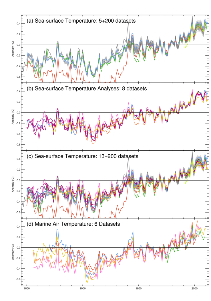
Figure 5: Global average sea-surface temperature anomalies and night marine air temperature anomalies from a range of data sets. (a) Simple gridded SST data sets including ICOADS v2.1 (red), 200 realizations of HadSST3 (pale grey), HadSST2 (dark green), TOHOKU (darker grey), ARC (Merchant et al. [2012] lime green) and the COBE-2 dataset sub-sampled to observational coverage (pale blue). (b) 8 Interpolated SST analyses including the COBE-2 dataset (pale blue), HadISST1.1 (gold), ERSSTv3b (orange), VBPCA, GPFA and GP (deep magenta), Kaplan (pink), NOCS (black). (c) shows the series in (a) and (b) combined. (d) NMAT: Ishii et al. (2005, red and blue), MOHMAT4N3 and HadMAT (Rayner et al. [2003], pink and orange), Berry and Kent [2009] (green), HadNMAT2 (Kent et al. [2013], gold).

Previous - 3.3.4 Refinements to Estimates of Pervasive Systematic Errors Index Next - 3.3.6 Summary of Pervasive Systematic Errors and Biases